
[Python] Numpy
Published:
In this post, Numpy, Scipy, Matplotlib are introduced.
Source : cs231n
Numpy
Numpy is the core library for scientific computing in Python. It provides a high-performance multidimensional array object, and tools for working with these arrays. If you are already familiar with MATLAB, you might find this tutorial useful to get started with Numpy.
- Initialization
import numpy as np

a = np.array([1, 2, 3])   # Create a rank 1 array
print(type(a))            # Prints "<class 'numpy.ndarray'>"
print(a.shape)            # Prints "(3,)"
print(a[0], a[1], a[2])   # Prints "1 2 3"
a[0] = 5                  # Change an element of the array
print(a)                  # Prints "[5, 2, 3]"

b = np.array([[1,2,3],[4,5,6]])    # Create a rank 2 array
print(b.shape)                     # Prints "(2, 3)"
print(b[0, 0], b[0, 1], b[1, 0])   # Prints "1 2 4"
a = np.zeros((2,2))   # Create an array of all zeros
print(a)              # Prints "[[ 0.  0.]
                      #          [ 0.  0.]]"

b = np.ones((1,2))    # Create an array of all ones
print(b)              # Prints "[[ 1.  1.]]"

c = np.full((2,2), 7)  # Create a constant array
print(c)               # Prints "[[ 7.  7.]
                       #          [ 7.  7.]]"

d = np.eye(2)         # Create a 2x2 identity matrix
print(d)              # Prints "[[ 1.  0.]
                      #          [ 0.  1.]]"

e = np.random.random((2,2))  # Create an array filled with random values
print(e)                     # Might print "[[ 0.91940167  0.08143941]
                             #               [ 0.68744134  0.87236687]]"
- Indexing - Slicing
# Create the following rank 2 array with shape (3, 4)
# [[ 1  2  3  4]
#  [ 5  6  7  8]
#  [ 9 10 11 12]]
a = np.array([[1,2,3,4], [5,6,7,8], [9,10,11,12]])

# Use slicing to pull out the subarray consisting of the first 2 rows
# and columns 1 and 2; b is the following array of shape (2, 2):
# [[2 3]
#  [6 7]]
b = a[:2, 1:3]

# A slice of an array is a view into the same data, so modifying it
# will modify the original array.
print(a[0, 1])   # Prints "2"
b[0, 0] = 77     # b[0, 0] is the same piece of data as a[0, 1]
print(a[0, 1])   # Prints "77"
You can also mix integer indexing with slice indexing. However, doing so will yield an array of lower rank than the original array. Note that this is quite different from the way that MATLAB handles array slicing:
# Create the following rank 2 array with shape (3, 4)
# [[ 1  2  3  4]
#  [ 5  6  7  8]
#  [ 9 10 11 12]]
a = np.array([[1,2,3,4], [5,6,7,8], [9,10,11,12]])

# Two ways of accessing the data in the middle row of the array.
# Mixing integer indexing with slices yields an array of lower rank,
# while using only slices yields an array of the same rank as the
# original array:
row_r1 = a[1, :]    # Rank 1 view of the second row of a
row_r2 = a[1:2, :]  # Rank 2 view of the second row of a
print(row_r1, row_r1.shape)  # Prints "[5 6 7 8] (4,)"
print(row_r2, row_r2.shape)  # Prints "[[5 6 7 8]] (1, 4)"

# We can make the same distinction when accessing columns of an array:
col_r1 = a[:, 1]
col_r2 = a[:, 1:2]
print(col_r1, col_r1.shape)  # Prints "[ 2  6 10] (3,)"
print(col_r2, col_r2.shape)  # Prints "[[ 2]
                             #          [ 6]
                             #          [10]] (3, 1)"
Indexing - Integer array indexing
When you index into numpy arrays using slicing, the resulting array view will always be a subarray of the original array. In contrast, integer array indexing allows you to construct arbitrary arrays using the data from another array. Here is an example:
a = np.array([[1,2], [3, 4], [5, 6]])

# An example of integer array indexing.
# The returned array will have shape (3,) and
print(a[[0, 1, 2], [0, 1, 0]])  # Prints "[1 4 5]"

# The above example of integer array indexing is equivalent to this:
print(np.array([a[0, 0], a[1, 1], a[2, 0]]))  # Prints "[1 4 5]"

# When using integer array indexing, you can reuse the same
# element from the source array:
print(a[[0, 0], [1, 1]])  # Prints "[2 2]"

# Equivalent to the previous integer array indexing example
print(np.array([a[0, 1], a[0, 1]]))  # Prints "[2 2]"
One useful trick with integer array indexing is selecting or mutating one element from each row of a matrix:
# Create a new array from which we will select elements
a = np.array([[1,2,3], [4,5,6], [7,8,9], [10, 11, 12]])

print(a)  # prints "array([[ 1,  2,  3],
          #                [ 4,  5,  6],
          #                [ 7,  8,  9],
          #                [10, 11, 12]])"

# Create an array of indices
b = np.array([0, 2, 0, 1])

# Select one element from each row of a using the indices in b
print(a[np.arange(4), b])  # Prints "[ 1  6  7 11]"

# Mutate one element from each row of a using the indices in b
a[np.arange(4), b] += 10

print(a)  # prints "array([[11,  2,  3],
          #                [ 4,  5, 16],
          #                [17,  8,  9],
          #                [10, 21, 12]])
- Boolean array indexing
a = np.array([[1,2], [3, 4], [5, 6]])

bool_idx = (a > 2)   # Find the elements of a that are bigger than 2;
                     # this returns a numpy array of Booleans of the same
                     # shape as a, where each slot of bool_idx tells
                     # whether that element of a is > 2.

print(bool_idx)      # Prints "[[False False]
                     #          [ True  True]
                     #          [ True  True]]"

# We use boolean array indexing to construct a rank 1 array
# consisting of the elements of a corresponding to the True values
# of bool_idx
print(a[bool_idx])  # Prints "[3 4 5 6]"

# We can do all of the above in a single concise statement:
print(a[a > 2])     # Prints "[3 4 5 6]"
- Datatypes
x = np.array([1, 2])   # Let numpy choose the datatype
print(x.dtype)         # Prints "int64"

x = np.array([1.0, 2.0])   # Let numpy choose the datatype
print(x.dtype)             # Prints "float64"

x = np.array([1, 2], dtype=np.int64)   # Force a particular datatype
print(x.dtype)                         # Prints "int64"
- array math
x = np.array([[1,2],[3,4]], dtype=np.float64)
y = np.array([[5,6],[7,8]], dtype=np.float64)

# Elementwise sum; both produce the array
# [[ 6.0  8.0]
#  [10.0 12.0]]
print(x + y)
print(np.add(x, y))

# Elementwise difference; both produce the array
# [[-4.0 -4.0]
#  [-4.0 -4.0]]
print(x - y)
print(np.subtract(x, y))

# Elementwise product; both produce the array
# [[ 5.0 12.0]
#  [21.0 32.0]]
print(x * y)
print(np.multiply(x, y))

# Elementwise division; both produce the array
# [[ 0.2         0.33333333]
#  [ 0.42857143  0.5       ]]
print(x / y)
print(np.divide(x, y))

# Elementwise square root; produces the array
# [[ 1.          1.41421356]
#  [ 1.73205081  2.        ]]
print(np.sqrt(x))
Note that unlike MATLAB, * is elementwise multiplication, not matrix multiplication. We instead use the dotfunction to compute inner products of vectors, to multiply a vector by a matrix, and to multiply matrices. dot is available both as a function in the numpy module and as an instance method of array objects:
x = np.array([[1,2],[3,4]])
y = np.array([[5,6],[7,8]])

v = np.array([9,10])
w = np.array([11, 12])

# Inner product of vectors; both produce 219
print(v.dot(w))
print(np.dot(v, w))

# Matrix / vector product; both produce the rank 1 array [29 67]
print(x.dot(v))
print(np.dot(x, v))

# Matrix / matrix product; both produce the rank 2 array
# [[19 22]
#  [43 50]]
print(x.dot(y))
print(np.dot(x, y))
Numpy provides many useful functions for performing computations on arrays; one of the most useful is sum:
x = np.array([[1,2],[3,4]])

print(np.sum(x))  # Compute sum of all elements; prints "10"
print(np.sum(x, axis=0))  # Compute sum of each column; prints "[4 6]"
print(np.sum(x, axis=1))  # Compute sum of each row; prints "[3 7]"
Apart from computing mathematical functions using arrays, we frequently need to reshape or otherwise manipulate data in arrays. The simplest example of this type of operation is transposing a matrix; to transpose a matrix, simply use the T attribute of an array object:
x = np.array([[1,2], [3,4]])
print(x)    # Prints "[[1 2]
            #          [3 4]]"
print(x.T)  # Prints "[[1 3]
            #          [2 4]]"

# Note that taking the transpose of a rank 1 array does nothing:
v = np.array([1,2,3])
print(v)    # Prints "[1 2 3]"
print(v.T)  # Prints "[1 2 3]"
Broadcasting
Broadcasting is a powerful mechanism that allows numpy to work with arrays of different shapes when performing arithmetic operations. Frequently we have a smaller array and a larger array, and we want to use the smaller array multiple times to perform some operation on the larger array.
For example, suppose that we want to add a constant vector to each row of a matrix. We could do it like this:
# We will add the vector v to each row of the matrix x,
# storing the result in the matrix y
x = np.array([[1,2,3], [4,5,6], [7,8,9], [10, 11, 12]])
v = np.array([1, 0, 1])
y = np.empty_like(x)   # Create an empty matrix with the same shape as x

# Add the vector v to each row of the matrix x with an explicit loop
for i in range(4):
    y[i, :] = x[i, :] + v

# Now y is the following
# [[ 2  2  4]
#  [ 5  5  7]
#  [ 8  8 10]
#  [11 11 13]]
print(y)
This works; however when the matrix x is very large, computing an explicit loop in Python could be slow. Note that adding the vector v to each row of the matrix x is equivalent to forming a matrix vv by stacking multiple copies of v vertically, then performing elementwise summation of x and vv. We could implement this approach like this:
# We will add the vector v to each row of the matrix x,
# storing the result in the matrix y
x = np.array([[1,2,3], [4,5,6], [7,8,9], [10, 11, 12]])
v = np.array([1, 0, 1])
vv = np.tile(v, (4, 1))   # Stack 4 copies of v on top of each other
print(vv)                 # Prints "[[1 0 1]
                          #          [1 0 1]
                          #          [1 0 1]
                          #          [1 0 1]]"
y = x + vv  # Add x and vv elementwise
print(y)  # Prints "[[ 2  2  4
          #          [ 5  5  7]
          #          [ 8  8 10]
          #          [11 11 13]]"
Numpy broadcasting allows us to perform this computation without actually creating multiple copies of v. Consider this version, using broadcasting:
# We will add the vector v to each row of the matrix x,
# storing the result in the matrix y
x = np.array([[1,2,3], [4,5,6], [7,8,9], [10, 11, 12]])
v = np.array([1, 0, 1])
y = x + v  # Add v to each row of x using broadcasting
print(y)  # Prints "[[ 2  2  4]
          #          [ 5  5  7]
          #          [ 8  8 10]
          #          [11 11 13]]"
Broadcasting two arrays together follows these rules:
If the arrays do not have the same rank, prepend the shape of the lower rank array with 1s until both shapes have the same length. (두 배열의 차원 수(rank)가 다르면차원이 더 작은 배열의 shape 앞에 1을 붙여서 차원 수를 맞춘다.)
A.shape = (3, 4)
B.shape = (4,)
B.shape → (1, 4)
The two arrays are said to be compatible in a dimension if they have the same size in the dimension, or if one of the arrays has size 1 in that dimension. (각 차원마다 다음 중 하나면 호환 가능: 두 배열의 크기가 같다 /한쪽의 크기가 1 )
(3, 4)
(1, 4)  → 호환 가능

(3, 4)
(2, 4)  → 첫 번째 차원에서 호환 불가
The arrays can be broadcast together if they are compatible in all dimensions. (모든 차원에서 위 조건을 만족해야 연산 가능)
After broadcasting, each array behaves as if it had shape equal to the elementwise maximum of shapes of the two input arrays. (브로드캐스팅 결과의 shape은 각 차원별로 두 배열 중 큰 값)
A: (3, 4)
B: (1, 4)
→ 결과 shape: (3, 4)
In any dimension where one array had size 1 and the other array had size greater than 1, the first array behaves as if it were copied along that dimension
A = np.array([[1],
              [2],
              [3]])   # shape (3,1)

B = np.array([10, 20, 30, 40])  # shape (4,)

A → (3,1)
B → (1,4)

A behaves like:
[[1, 1, 1, 1],
 [2, 2, 2, 2],
 [3, 3, 3, 3]]

B behaves like:
[[10, 20, 30, 40],
 [10, 20, 30, 40],
 [10, 20, 30, 40]]
Here are some applications of broadcasting:
# Compute outer product of vectors
v = np.array([1,2,3])  # v has shape (3,)
w = np.array([4,5])    # w has shape (2,)
# To compute an outer product, we first reshape v to be a column
# vector of shape (3, 1); we can then broadcast it against w to yield
# an output of shape (3, 2), which is the outer product of v and w:
# [[ 4  5]
#  [ 8 10]
#  [12 15]]
print(np.reshape(v, (3, 1)) * w)

# Add a vector to each row of a matrix
x = np.array([[1,2,3], [4,5,6]])
# x has shape (2, 3) and v has shape (3,) so they broadcast to (2, 3),
# giving the following matrix:
# [[2 4 6]
#  [5 7 9]]
print(x + v)

# Add a vector to each column of a matrix
# x has shape (2, 3) and w has shape (2,).
# If we transpose x then it has shape (3, 2) and can be broadcast
# against w to yield a result of shape (3, 2); transposing this result
# yields the final result of shape (2, 3) which is the matrix x with
# the vector w added to each column. Gives the following matrix:
# [[ 5  6  7]
#  [ 9 10 11]]
print((x.T + w).T)
# Another solution is to reshape w to be a column vector of shape (2, 1);
# we can then broadcast it directly against x to produce the same
# output.
print(x + np.reshape(w, (2, 1)))

# Multiply a matrix by a constant:
# x has shape (2, 3). Numpy treats scalars as arrays of shape ();
# these can be broadcast together to shape (2, 3), producing the
# following array:
# [[ 2  4  6]
#  [ 8 10 12]]
print(x * 2)
SciPy
Numpy provides a high-performance multidimensional array and basic tools to compute with and manipulate these arrays. SciPy builds on this, and provides a large number of functions that operate on numpy arrays and are useful for different types of scientific and engineering applications.
Image operations
SciPy provides some basic functions to work with images. For example, it has functions to read images from disk into numpy arrays, to write numpy arrays to disk as images, and to resize images. Here is a simple example that showcases these functions:
from scipy.misc import imread, imsave, imresize

# Read an JPEG image into a numpy array
img = imread('assets/cat.jpg')
print(img.dtype, img.shape)  # Prints "uint8 (400, 248, 3)"

# We can tint the image by scaling each of the color channels
# by a different scalar constant. The image has shape (400, 248, 3);
# we multiply it by the array [1, 0.95, 0.9] of shape (3,);
# numpy broadcasting means that this leaves the red channel unchanged,
# and multiplies the green and blue channels by 0.95 and 0.9
# respectively.
img_tinted = img * [1, 0.95, 0.9]

# Resize the tinted image to be 300 by 300 pixels.
img_tinted = imresize(img_tinted, (300, 300))

# Write the tinted image back to disk
imsave('assets/cat_tinted.jpg', img_tinted)
Distance between points
The function
scipy.spatial.distance.pdistcomputes the distance between all pairs of points in a given set:
import numpy as np
from scipy.spatial.distance import pdist, squareform

# Create the following array where each row is a point in 2D space:
# [[0 1]
#  [1 0]
#  [2 0]]
x = np.array([[0, 1], [1, 0], [2, 0]])
print(x)

# Compute the Euclidean distance between all rows of x.
# d[i, j] is the Euclidean distance between x[i, :] and x[j, :],
# and d is the following array:
# [[ 0.          1.41421356  2.23606798]
#  [ 1.41421356  0.          1.        ]
#  [ 2.23606798  1.          0.        ]]
d = squareform(pdist(x, 'euclidean'))
print(d)
Matplotlib
Matplotlib is a plotting library.
Plotting
The most important function in matplotlib is
plot, which allows you to plot 2D data. Here is a simple example:
import numpy as np
import matplotlib.pyplot as plt

# Compute the x and y coordinates for points on a sine curve
x = np.arange(0, 3 * np.pi, 0.1)
y = np.sin(x)

# Plot the points using matplotlib
plt.plot(x, y)
plt.show()  # You must call plt.show() to make graphics appear.
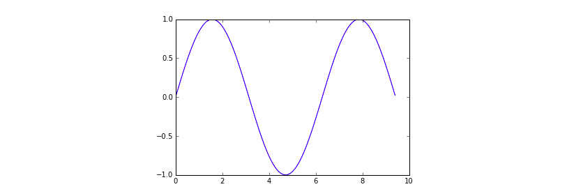
Running this code produces the following plot:
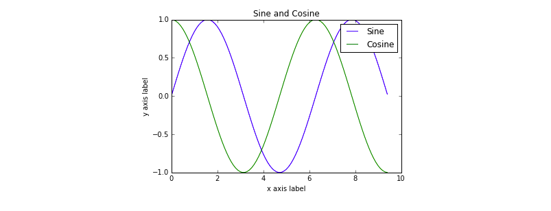
With just a little bit of extra work we can easily plot multiple lines at once, and add a title, legend, and axis labels:
import numpy as np
import matplotlib.pyplot as plt

# Compute the x and y coordinates for points on sine and cosine curves
x = np.arange(0, 3 * np.pi, 0.1)
y_sin = np.sin(x)
y_cos = np.cos(x)

# Plot the points using matplotlib
plt.plot(x, y_sin)
plt.plot(x, y_cos)
plt.xlabel('x axis label')
plt.ylabel('y axis label')
plt.title('Sine and Cosine')
plt.legend(['Sine', 'Cosine'])
plt.show()
Subplots
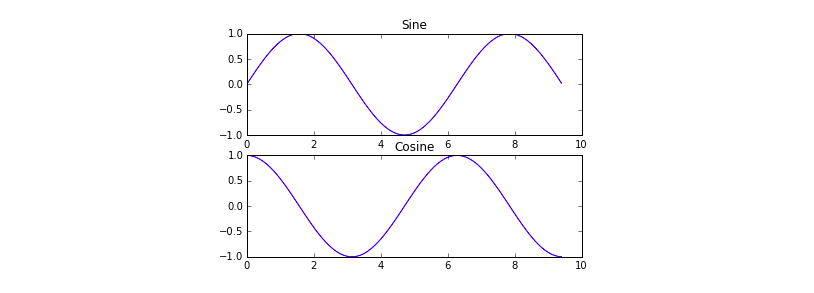
You can plot different things in the same figure using the
subplotfunction. Here is an example:
import numpy as np
import matplotlib.pyplot as plt

# Compute the x and y coordinates for points on sine and cosine curves
x = np.arange(0, 3 * np.pi, 0.1)
y_sin = np.sin(x)
y_cos = np.cos(x)

# Set up a subplot grid that has height 2 and width 1,
# and set the first such subplot as active.
plt.subplot(2, 1, 1)

# Make the first plot
plt.plot(x, y_sin)
plt.title('Sine')

# Set the second subplot as active, and make the second plot.
plt.subplot(2, 1, 2)
plt.plot(x, y_cos)
plt.title('Cosine')

# Show the figure.
plt.show()
Images
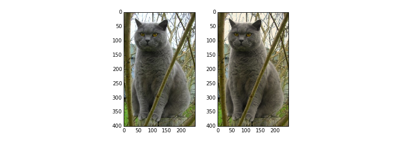
You can use the
imshowfunction to show images. Here is an example:
import numpy as np
from scipy.misc import imread, imresize
import matplotlib.pyplot as plt

img = imread('assets/cat.jpg')
img_tinted = img * [1, 0.95, 0.9]

# Show the original image
plt.subplot(1, 2, 1)
plt.imshow(img)

# Show the tinted image
plt.subplot(1, 2, 2)

# A slight gotcha with imshow is that it might give strange results
# if presented with data that is not uint8. To work around this, we
# explicitly cast the image to uint8 before displaying it.
plt.imshow(np.uint8(img_tinted))
plt.show()
Leave a Comment